
Device guide
tinySA Ultra: reading a spectrum and testing a reference
Learn frequency, amplitude, dBm, resolution and sweeping through a CAL reference exercise, illustrative plots and practical interpretation criteria.
What appears on the screen
A peak on a spectrum analyzer starts an investigation: a response exists at a particular frequency, level and configuration. The reading becomes useful when those conditions are known. The tinySA Ultra lets you study that relationship on a bench with a controlled reference before observing signals in the environment.
Start with identification: tinySA Ultra is the available name, but this unit’s revision, firmware and accessories have not yet been documented. The official comparison distinguishes Ultra ZS405 from Ultra+ ZS406/ZS407, with differences in coverage and performance. Before following a setting, check the front, label and version information; do not transfer specifications between variants.[1]
We will follow the documented Ultra-family architecture and prepare a 30 MHz exercise. Use the plots and table to work through the reasoning: their numbers are illustrative and do not come from measurements of the laboratory unit.
From the input to the trace
In the documented heterodyne architecture, a signal enters the RF connector, passes through a choice of attenuation or amplification, and continues through filters and frequency conversions. A local oscillator sweeps the selected range. After resolution filtering, a detector measures the level. The display combines those observations into a frequency-versus-amplitude trace.[2]
This sequence explains a useful distinction: the plot is built during a sweep. Points at different frequencies can correspond to different times. A short emission may occur while the instrument is observing another region. A single trace therefore does not show everything that happened in the environment simultaneously.
Frequency, span and resolution
The horizontal axis shows frequency. You can specify start and stop, or a center and span, the total displayed width. A 30 MHz center with a 20 MHz span gives a window from 20 to 40 MHz. Reducing span enlarges the region of interest on the display; it does not, by itself, create additional ability to separate signals.
RBW, resolution bandwidth, defines the filter used for the observation. A smaller RBW helps examine nearby details but can increase sweep time. The project documents limitations involving resolution, noise, spurious responses and wide signals in Ultra mode. Those limitations belong alongside the interpretation.[3]
Amplitude: dBm and dB
dBm expresses power relative to 1 milliwatt: P(dBm) = 10 × log10(P / 1 mW). dB expresses a ratio. For example, −40 dBm is 20 dB above −60 dBm, a power ratio of 100. The minus sign does not mean there is no energy; it indicates power below the 1 mW reference.
The observed level belongs to the measurement path, including connections and settings. With an antenna, do not treat it as the transmitter’s total output power. In a comparison, write the unit, RBW, attenuation and source state alongside the result.
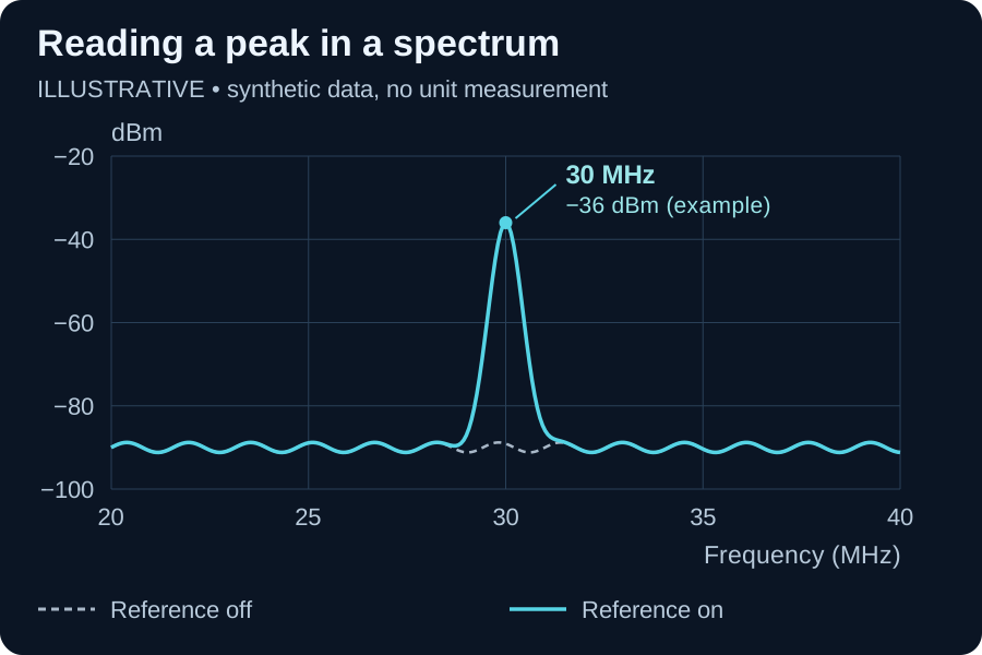
Teaching plot with synthetic data to help you follow the reading. Peak height and width do not specify tinySA performance.
Controls worth understanding first
The consulted menu documentation describes firmware 1.3507 or later; option locations can differ on your unit. Use these names as references and verify the matching version.[4]
| Documented control | Question it helps answer |
|---|---|
| CENTER / SPAN | Which frequency region am I observing? |
| REF LEVEL / SCALE/DIV | How is level distributed vertically? |
| RBW | Which resolution was selected for this sweep? |
| ATTENUATE / LNA | How is the signal conditioned before measurement? |
| MARKER | Which frequency and level do I want to record? |
| MAX HOLD | What is the largest stored value at each point? |
Attenuating the input and changing the vertical scale are different operations. The first changes the signal path; the second changes presentation. MAX HOLD keeps previous maxima, so reset it when comparing a new condition. For the first exercise, use a normal trace without accumulation.[4]
Laboratory: observe the CAL output
Objective: recognize a known reference, change the viewing window and document the difference. CAL is a reference generator output separate from the RF connector; Ultra documentation includes a 30 MHz selection. This provides a more controlled setup than starting with an antenna in the environment.[5]
Prepare the identified unit and a suitable short SMA cable. Before connecting them, check the revision’s input limits and matching procedure. Do not connect a power transmitter’s output directly to the instrument. Official specifications distinguish attenuation, LNA and maximum levels; an absolute limit is not an operating target.[6]
-
Record the starting state. Note model, version, power arrangement and calibration status. Preserve settings used for other work.
-
Connect the reference and run the self-test. After confirming output functions, connect CAL to RF with the short cable. With the cable connected, run
CONFIG → SELF TESTaccording to the revision’s documentation. If a test fails, record and resolve it before continuing. A successful self-test does not replace traceable calibration. After completing it, return to spectrum analyzer mode; CAL has its own control.[4][5] -
Set the exercise window. Use a 30 MHz center, 20 MHz span and dBm units. If these settings are available on the revision, leave LNA off, use 10 dB attenuation and automatic RBW. These are teaching choices for this reference, not a universal configuration.
-
Observe the setup’s background. Disable CAL and record a normal trace. Note the actual RBW, scale and observation time. This is the background for this connection, not a universal measurement of internal noise.
-
Enable the 30 MHz reference. Wait for complete sweeps. Place a marker in the reference region and record frequency and level. Look for repeatability; do not adjust calibration to force agreement with the illustrative table.
-
Change only span. Reduce it to 2 MHz while retaining the 30 MHz center. Check whether automatic RBW changed. To compare span alone, select a manual RBW supported in both windows and repeat both observations.
-
Explore resolution. Within the same window, compare two available RBWs and record sweep time and trace shape. The question is how observation changes, not which setting makes the most impressive peak.
-
Repeat off / on / off. Return to the recorded configuration before each cycle. Save traces when storage is available, or photograph the screen with its parameters. Finish by disabling CAL and restoring the state needed for the next task.
Recording the results
ILLUSTRATIVE table, with no real measurements. The values are not a specification, acceptance tolerance or calibration certificate.
| Condition | Window | Illustrative reading at 30 MHz | Example conclusion |
|---|---|---|---|
| CAL disabled | 20–40 MHz | Background near −90 dBm | No prominent reference peak |
| CAL at 30 MHz | 20–40 MHz | Peak at −36 dBm | Reference distinguishable from background |
| Same CAL, smaller window | 29–31 MHz | Peak at −36 dBm | Expanded position, similar level |
| CAL disabled again | 20–40 MHz | Return to background | The change followed the reference |
If a peak persists after disabling CAL, first check for a frozen trace or MAX HOLD. If shape changes substantially with attenuation or LNA, investigate configuration and possible overload. The manufacturer documents that enabling LNA disables the internal attenuator and can make overload from strong signals easier.[3]
What to take into a real assessment
A useful record includes source, connection, revision, firmware, range, RBW, attenuation, LNA state and trace. Also record what was outside the observation. A peak still does not identify the protocol, contents or person responsible for an emission; an absent peak applies only within the verified conditions.
Use the reference to learn the instrument. Then formulate a specific field question and document a suitable setup. To compare announcements from known access points, the ESP32 Marauder inventory guide develops a different layer of observation.
References
-
tinySA. tinySA model comparison table. Wiki, TinySA4. Ultra/Ultra+ identification and differences between variants. Source. Accessed 17 October 2026. ↩
-
tinySA. tinySA Ultra Technical Description. 2023. Input path and frequency-conversion and detection architecture. Source. Accessed 17 October 2026. ↩
-
tinySA. Limitations. Wiki, TinySA4. Resolution, sweeping, spurious responses and overload. Source. Accessed 17 October 2026. ↩ ↩2
-
tinySA. Mode Menu. Wiki, TinySA4. Analyzer mode and CAL reference-output control. Source. Accessed 17 October 2026. ↩ ↩2
-
tinySA. Specification. Wiki, TinySA4. Electrical limits and input conditions. Source. Accessed 17 October 2026. ↩